Continual Learning and Memory (2): Memory Architecture in Language Models

In our first post, we recapped the formulations of two continual learning papers. Both approaches conduct test-time learning to compress raw input into model parameters, effectively using those parameters as a dynamic working memory. In this post, we step back to examine the evolution of language models through the lens of memory.

TLDR: Everything is memory. Ultimately, the evolution of language models boils down to two design choices: (1) How will you represent the memory (vectors, matrices, weights, or external pools)? and (2) How will you update it (appending, closed-form optimization, or gradient descent)?

Recurrent Hidden Vector as Memory

The concept of “memory” in neural networks is far from new. Recurrent Neural Networks (RNNs) have long utilized a hidden state vector to carry information over to new timesteps (or tokens, in modern terminology). The Long Short-Term Memory (LSTM) architecture explicitly formalized this by distinguishing between a “hidden state” (output) and a “cell state” (memory).

At a high level, we can view the memory update as $c_t=f(x_t, c_{t-1})$, where $c_t$ and $c_{t-1}$ represent the memory at the current and previous timesteps, and $x_t$ is the current input. LSTMs introduce a forget gate and an input gate to regulate how much of the past memory $c_{t-1}$ is retained and how much new information from $x_t$ is added.

In theory, this recurrent memory allows information to be carried over indefinitely—from previous tasks to new ones. Aha! It turns out we had long-context language models for continual learning over 30 years ago.

However, it has two practical issues:

(1) Capacity: A fixed-length hidden vector is easily overloaded; it simply cannot losslessly store the vast amount of information contained in a long sequence.

(2) Permanence of Loss: Once information is discarded via the forget mechanism, it is gone forever. The model cannot “look back” to retrieve it later.

Attention-based Memory

Quadratic Attention as Memory

The first modern attention paper, proposed a solution: keep the RNN hidden vectors for all encoded tokens and use an attention mechanism to search over them during decoding. (Note: This was originally an encoder-decoder framework for machine translation, distinct from today’s decoder-only LLMs). This RNN + Attention architecture effectively utilizes two types of memory: (1) RNN hidden state, which is a fixed-size vector representing compressed context, (2) token activations, which form a growing buffer of states with a size linear to the input length.

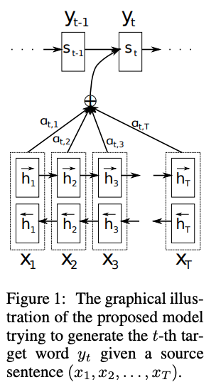
This mechanism laid the groundwork for the standard attention found in Transformers, which relies exclusively on this retrieved history as its working memory.

where $q,k \in \mathbb{R}^{d_k}$, $v \in \mathbb{R}^{d_v}$, and $W_q, W_k, W_v$ are projection matrices.

Because Transformer attention provides a direct, lossless view of all past tokens, the recurrent hidden state became obsolete as a working memory. However, this capability comes at a steep price: quadratic time complexity with respect to sequence length.

Linear Attention (Recurrent Hidden Matrix) as Memory

The Linear Attention paper addresses this bottleneck by removing the softmax normalization from the attention mechanism. It observes that for any non-negative similarity function $\text{sim}(q_t, k_j)$, including softmax, there exists a feature map $\phi$ (potentially in infinite dimensions) such that $\text{sim}(q_t, k_j)=\phi(q_t)^\top\phi(k_j)$. Under this formulation, attention can be rewritten as:

For simplicity, if we use the identity function as the feature map $\phi$ and omit the denominator normalization, the equation simplifies to:

Here, the term $\sum_{j=1}^{t} k_j v_j^\top$ can be denoted as a matrix $S_t \in \mathbb{R}^{d_k \times d_v}$. Crucially, this matrix can be computed recurrently:

This brings us full circle: $S_t$ acts as a recurrent memory, much like the RNN hidden vector. However, we are now using a matrix rather than a vector. While significantly more powerful than a simple vector, this compression is still lossy compared to standard Transformers.

Consider retrieving a specific value $v_i$ using its key $k_i$:

If all keys are normalized to unit length, this becomes:

To minimize retrieval error (i.e., reduce the noise term to zero), all keys must be orthogonal. This implies that a matrix of dimension $d_k$ can only losslessly store up to $d_k$ distinct items.

Gated DeltaNet

To mitigate the lossy nature of Linear Attention, researchers revisited the LSTM’s forget gate, leading to Gated Linear Attention. By introducing an input-dependent gate $G_t$, the model can selectively “clear up space” in $S_t$ for new information.

Furthermore, DeltaNet argues that the update rule should be mindful of what is already stored. Instead of blindly adding $k_t v_t^\top$, we should only add the difference (or delta) between the new information and the existing memory. Conceptually, we first “erase” the old value associated with $k_t$ and then write the new value¹:

where $v_{old}^\top=k_t^\top S_{t-1}$. Expanding this term yields:

Interestingly, this update rule is equivalent to one step of gradient descent on an L2 loss function that measures the reconstruction error of the key-value pair:

From this perspective, Linear Attention is effectively a closed-form solution for test-time training of the memory matrix:

Moreover, the Gated Linear Attention can be viewed as a weight decay and combined into this optimization. The combined Gated DeltaNets are then used in modern LLMs such as Kimi, Qwen3-next.

Feed-Forward Networks as Memory

The rise of Linear Attention and DeltaNet shifts our perspective on how attention mechanisms operate. In standard Transformers, attention is commonly viewed as working memory retrieval over a dynamically generated list of activations, updated by growing activation buffers.

But now we can reframe this: attention (the retrieval) acts as a function, while the memory pool update can be treated as an optimization problem. This reframing connects beautifully to an existing stream of research that interprets the Feed-Forward Network (FFN) layers in Transformers as a massive memory retrieval mechanism.

Mathematically, we can express the standard FFN operation as:

where $K, V \in \mathbb{R}^{d \times d_{ff}}$ are the projection matrices and $f$ is a non-linear activation function.

This formulation views the FFN as a memory layer containing $d_{ff}$ distinct key-value pairs. The FFN first maps the input $x$ against $d_{ff}$ memory keys, uses the non-linearity $f$ to select relevant keys, and then outputs a weighted average of the corresponding memory values. If we were to use a softmax function for the non-linearity $f$, the FFN would become mathematically identical to an attention-like memory lookup:

While original Transformers relied on ReLU activations for $f$, modern LLMs predominantly use gated activations, such as SwiGLU:

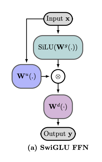
In this architecture, $W^u$ and $W^d$ conceptually correspond to the key ($K$) and value ($V$) projections from the earlier equation. In standard nomenclature, $W^u$, $W^d$, and $W^g$ represent the up-projection, down-projection, and gating weight matrices, respectively. This structure enables the model to selectively activate relevant memory keys using dedicated gating parameters ($W^g$) conditioned directly on the input $x$.

Typically, we view these FFN weights as static repositories for pre-training knowledge that remain fixed during inference. However, recent breakthroughs like Titans and TTT-E2E propose that FFNs can also serve as dynamic, mutable working memory, provided we introduce an efficient mechanism to optimize and update these weights at test time.

Sparse Memory Layers

Recently, the Memory Layers paper argued that memory access is inherently sparse: only a few relevant pieces of information need to be retrieved at any given time, while the vast majority of stored knowledge remains irrelevant to the current context. Consequently, the dense matrix multiplication used in Feed-Forward Network (FFN) layers is an inefficient architecture for storage and retrieval.

They propose replacing the dense FFN layers in Transformer blocks with a Memory Lookup Layer. This sparse architecture allows for storing millions of memory slots, orders of magnitude more than a standard FFN, while maintaining efficient retrieval.

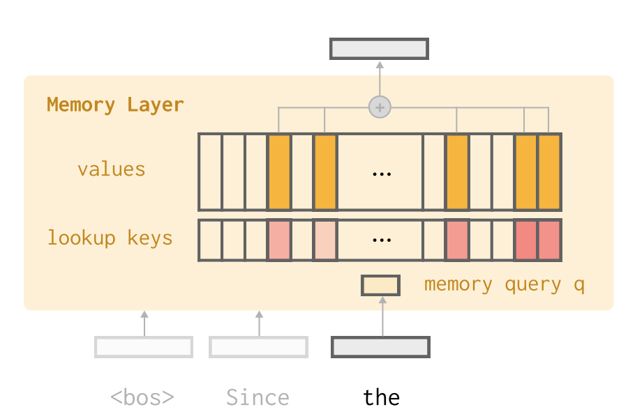
The memory layer contains a set of trainable parameters: keys $K \in \mathbb{R}^{d \times N}$ and values $V \in \mathbb{R}^{d \times N}$. Unlike the dynamic activations in attention, these parameters store static memory from pre-training data. At test time, a query $q \in \mathbb{R}^d$ is used to retrieve only the top-$k$ relevant keys ($k \ll N$), followed by a standard attention operation over just those $k$ slots:

External Memory Pool

While innovations in Linear Attention allow for more efficient reading and writing of the memory state $S$, these methods still consolidate all knowledge into a single, superimposed representation rather than maintained in individual, discrete memory records. An alternative approach is to utilize an external memory pool and interact with it in a similar fashion as attention. This line of research dates back over a decade; let’s briefly recap its evolution.

Following the rise of attention mechanisms in machine translation, researchers began to conceptualize neural memory as analogous to RAM in a computer, which is an external component that the CPU (the neural network) can read from and write to. Guided by this philosophy, pioneering works like Memory Networks and Neural Turing Machines implemented a memory pool $M \in \mathbb{R}^{N \times d}$ containing $N$ slots, each storing a $d$-dimensional vector. The model is then trained to learn specific read/write operations to manipulate this external pool for task-specific goals.

More recently, architectures like MemoryLLM have augmented the standard Transformer attention mechanism by maintaining a set of external memory vectors.

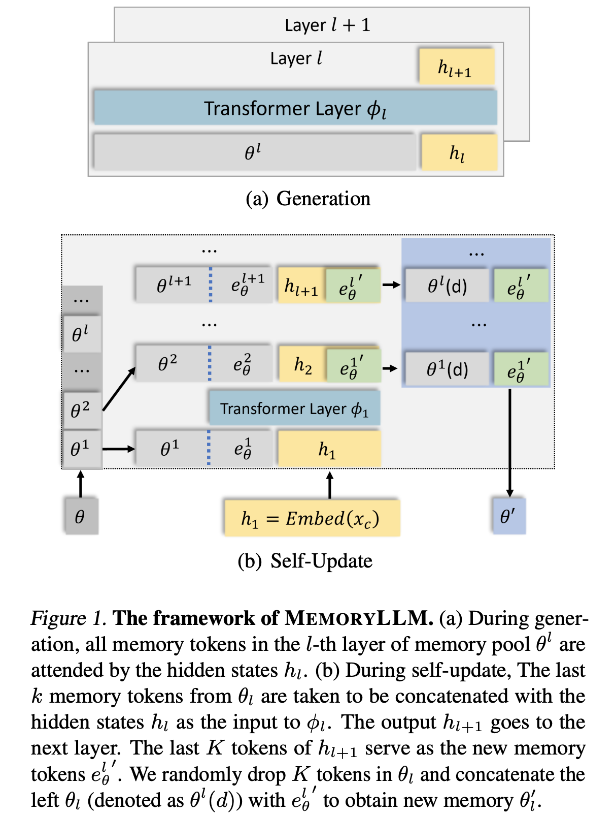
During generation, MemoryLLM attends to both the local context and the global memory pool, extending the standard formulation $Attention(Q, K, V)$ to: \(Attention(Q_X, [K_M;K_X], [V_M;V_X]),\) where $X$, $M$ represent the local context and global memory respectively.

Unlike the standard Attention, which updates the activations at every token, the MemoryLLM pool is updated only after processing a complete text segment (e.g., a paragraph). During this update phase, the model concatenates the hidden states of the new text chunk with the last $k$ records ($k \ll N$) from the existing memory pool. These are processed together, and the final $k$ hidden states are written back into the pool, replacing randomly selected vectors.

Conceptually, this acts as a “k-gram” conditional memory write: the model uses the previous $k$ memory records to condition the compression of the current text chunk into the latent memory space, generating $k$ updated vectors.

Wrap-up

We’ve traced memory in language models from fixed-size hidden vectors, through attention-based token buffers, to matrices updated via gradient descent, and finally to sparse and external memory pools. Despite their apparent diversity, these architectures all face the same fundamental trade-offs: capacity vs. efficiency, and lossless retrieval vs. compressive storage.

A recurring theme is that memory updates increasingly resemble optimization — DeltaNet’s update rule is literally a gradient step, and test-time training methods like Titans extend this idea to FFN weights.

References

1. Long Short-Term Memory [PDF] Hochreiter, Sepp and Schmidhuber, Jürgen, 1997.

2. Neural Machine Translation by Jointly Learning to Align and Translate [PDF] Bahdanau, Dzmitry, Cho, Kyunghyun, and Bengio, Yoshua, 2014.

3. Attention Is All You Need [PDF] Vaswani, Ashish, Shazeer, Noam, Parmar, Niki, Uszkoreit, Jakob, Jones, Llion, Gomez, Aidan N., Kaiser, Łukasz, and Polosukhin, Illia, 2017.

4. Transformers are RNNs: Fast Autoregressive Transformers with Linear Attention [PDF] Katharopoulos, Angelos, Vyas, Apoorv, Pappas, Nikolaos, and Fleuret, François, 2020.

5. Gated Linear Attention Transformers with Hardware-Efficient Training [PDF] Yang, Songlin, Wang, Bailin, Shen, Yikang, Panda, Rameswar, and Kim, Yoon, 2024.

6. Parallelizing Linear Transformers with the Delta Rule over Sequence Length [PDF] Yang, Songlin, Wang, Bailin, Zhang, Yu, Shen, Yikang, and Kim, Yoon, 2024.

7. Gated Delta Networks: Improving Mamba2 with Delta Rule [PDF] Yang, Songlin, Kautz, Jan, and Hatamizadeh, Ali, 2024.

8. Transformer feed-forward layers are key-value memories. [PDF] Geva, Mor, Roei Schuster, Jonathan Berant, and Omer Levy, 2021.

9. Titans: Learning to Memorize at Test Time [PDF] Behrouz, Ali, Zhong, Peilin, and Mirrokni, Vahab, 2024.

10. End-to-End Test-Time Training for Long Context [PDF] Tandon, Arnuv, Dalal, Karan, Li, Xinhao, Koceja, Daniel, Rød, Marcel, Buchanan, Sam, Wang, Xiaolong, et al., 2025.

11. Memory Layers at Scale [PDF] Mu, Zhihang, Qiu, Shun, Lin, Xien, Huang, Po-Yao, Yan, Yingwei, and Lei, Tao, 2024.

12. Memory Networks [PDF] Weston, Jason, Chopra, Sumit, and Bordes, Antoine, 2014.

13. Neural Turing Machines [PDF] Graves, Alex, Wayne, Greg, and Danihelka, Ivo, 2014.

14. MemoryLLM: Towards Self-Updatable Large Language Models [PDF] Wang, Yu, Dong, Yifan, Zeng, Zhuoyi, Ko, Shangchao, Li, Zhe, and Xiong, Wenhan, 2024.